Cluster Optimisation

Optimise points in 3d space based on a potential

CoM

 CoM (*vectors)

returns the CoM of vectors

source

CoMTransform

 CoMTransform (*vectors)

Transforms vectors so the CoM is at the origin

source

InertiaTensor

 InertiaTensor (*vectors)

returns the inertia tensor of 3D vectors

source

point_setup

 point_setup (n:int, seed:int=0)

returns n points distributed on the unit sphere

source

geom_opt

 geom_opt (points, F_calc, iterations=1000, factor=0.0001)

optimises geometry of points in 3D space using gradient descent

source

System

 System (n:int=7, function:str='(4*((1/r)^12 -(1/r)^6))')

A cluster system, defined by n points and a pairwise potential in term of r, given as a string

	Type	Default	Details
n	int	7	the number of atoms in the cluster
function	str	(4*((1/r)^12 -(1/r)^6))	the pairwise potential between any two atoms in the cluster

source

System.optimise

 System.optimise (riter:int=10000, giter:int=1000, gfactor:int=0.0001,
                  biter:int=100)

	Type	Default	Details
riter	int	10000	the number of random initial configurations to consider
giter	int	1000	the number of gradient descent iterations to consider
gfactor	int	0.0001	the factor for the gradient descent
biter	int	100	the number of basin hopping iterations to perform

Optimisation is done by random search, followed by gradient descent followed by using scipy’s basinhopping routine. For the Lennard Jones potential, the results have been checked against the Cambridge Cluster Database and are accurate for 6 decimal places up to \(n=10\)

lj7 = System(7)
lj7.optimise()

print(lj7)

Energy -16.505384, for 7 points

lj7.plot()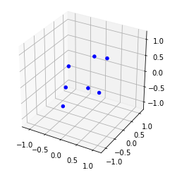

For the morse potential in the reduced form \[\exp(\rho_{0} (1-r))(\exp(\rho_{0} (1-r))-2)\] as given on the Cambridge Cluster Database, the results for \(\rho_{0} = (3,6,10,14)\) have been checked against the results on http://doye.chem.ox.ac.uk/jon/structures/Morse/tables.html and are accurate for 7 atoms to 6 dps. For 5 atoms, the results are identical for \(\rho_{0} = (6,10,14)\) but for \(\rho_{0} = 3\), smaller by 0.000001: likely a rounding error.

m7 = System(7, '(exp(3*(1-r)))*(exp(3*(1-r))-2)')
m7.optimise()

print(m7)

Energy -17.552961, for 7 points

m7.plot()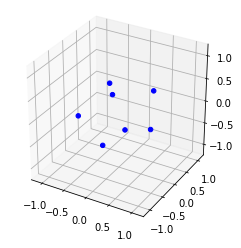

For 6 points, the value cannot be calculated directly for all but \(\rho = 3\). However, using this geometry as start point, all values can be calculated to within 0.000001.

m6 = System(6, '(exp(3*(1-r)))*(exp(3*(1-r))-2)')
m6.optimise()
print(m6, 'rho = 3')
m6.function = '(exp(6*(1-r)))*(exp(6*(1-r))-2)' # leave the points as previously optimised but change the pairwise potential
m6.optimise(riter=0) # do not do any random optimisation steps
print(m6, 'rho = 6')
m6.function = '(exp(10*(1-r)))*(exp(10*(1-r))-2)' # leave the points as previously optimised but change the pairwise potential
m6.optimise(riter=0) # do not do any random optimisation steps
print(m6, 'rho = 10')
m6.function = '(exp(14*(1-r)))*(exp(14*(1-r))-2)' # leave the points as previously optimised but change the pairwise potential
m6.optimise(riter=0) # do not do any random optimisation steps
print(m6, 'rho = 14')

Energy -13.544229, for 6 points rho = 3
Energy -12.487809, for 6 points rho = 6
Energy -12.094943, for 6 points rho = 10
Energy -12.018170, for 6 points rho = 14

source

System.xyz

 System.xyz (name:str=None)

Returns the coordinates of the system in .xyz format

	Type	Default	Details
name	str	None	name of file to save to: if None prints

The final configuration can be output in .xyz format

lj7.xyz()

7
Energy -16.505384, for 7 points, calculated by ChemII tools
He 0.3849546544 -0.1048571302 0.8689910322
He -0.2296806096 0.6400449466 -0.6722498078
He -0.5186360529 0.0632089849 0.2373778855
He 0.5186360103 -0.0632089496 -0.2373778974
He 0.2512385919 0.8659521341 0.3183340784
He -0.3931890427 -0.4703826180 -0.7338072527
He -0.0133235514 -0.9307573678 0.2187319618